The physiologic behavior of PET tracers is usually quite complex. A comprehensive model accurately describing its kinetics therefore requires many compartments and exchange parameters. However, as the PET signal is limited in quality and information, the model must be simplified to a degree that only a few parameters remain. When estimating a model with many parameters, the variance of the parameter estimates tends to be very high, so that a reliable interpretation of the results becomes impossible. A simplified model with fewer parameters will provide more precise results, but these parameters may be biased. Therefore, the optimal trade-off between bias and uncertainty has to be sought by testing models of decreasing complexity.
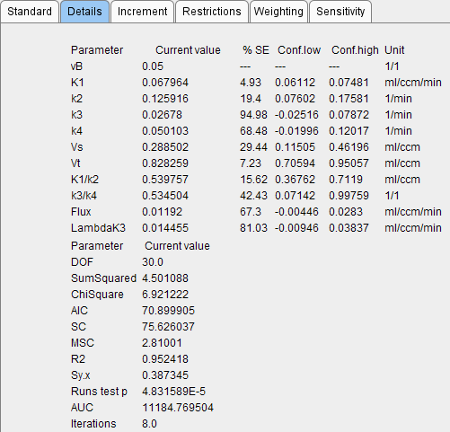
After every model fit detailed information about the parameter estimates and the goodness-of-fit is available on the Details tab.

Parameter Standard Error
Nonlinear regression using the Levenberg-Marquardt optimization reports a standard error (SE) for each fitted parameter value. The SE is calculated by multiplying the diagonal elements of the covariance matrix obtained by the fit with Chi Square and taking the square root. Note that SE is displayed as % of the actual parameter value.
Calculation of the macroparameter SE involves the covariance matrix and the partial derivatives at the solution. Example of the SE calculation for Vs of the 2-Tissue compartment model (Vs=K1k3/k2k4):
if (k2k4 > 0) { // Calculation of the the partial derivatives (pder) of Vs at the solution
pder[K1_IND] = k3 / k2k4;
pder[K2_IND] = -K1 * k3 / (k2 * k2k4);
pder[K3_IND] = K1 / k2k4;
pder[K4_IND] = -K1 * k3 / (k4 * k2k4);
variance = varianceFromModelCovar(pder, covar); // matrix multiplication: pder_transverse*covar*pder
SE = sqrt(variance*chiSqr);
}
The reason why the SE of a macroparameter can be lower than that of the parameters involved in the calculation is that the parameters are correlated.
Parameter Confidence Intervals
If the inherent fitting assumptions are true, a 95% confidence interval can be approximated by the result parameter plus/minus two standard errors. This confidence interval is displayed for each fitted parameter (Conf.low, Conf.high).
There will be a 95% chance that the confidence interval contains the true parameter value. A sufficiently narrow confidence interval indicates that the parameter could be determined with a reasonable certainty, whereas a wide interval makes it necessary to revise the configuration of the used model, or look for a more appropriate model.
Goodness-of-Fit
The following measures are defined which allow a direct or indirect assessment of the goodness-of-fit:
DOF |
Degrees of freedom defined as the number of valid measurements minus the number of fitted parameters. |
SumSquared |
Sum of squared (unweighted) residuals. |
ChiSquare |
Reduced Chi square. Sum of squared, weighted residuals, divided by the degrees of freedom. The reduced chi-square provides a useful measure of goodness-of-fit. If the model describes the measured data, the reduced chi-square will mostly represent the variance of the data and will be close to 1.0 (when weighting is appropriate). |
AIC |
Akaike Information Criterion. The AIC methodology attempts to find the model that best explains the data with a minimum of free parameters. The AIC is calculated with the second order correction for small sample size (<40). The preferred model is the one with the lowest AIC value. |
SC |
Schwartz Criterion, also called Bayesian Information Criterion (BIC). The preferred model is the one with the lowest SC value. |
MSC |
Another criterion used in the Scientist Software (MicroMath, Saint Louis, Missouri USA) is the Model Selection Criterion. The preferred model is the one with the highest MSC value. |
R2 |
There is also a measure of the goodness-of-fit, the coefficient of determinationR2, a number between 0 and 1. A value of 0 means that the fit is not better than a horizontal line through the mean of all measurements, whereas a value of 1 means that all measurements lie exactly on the curve. High R2 values indicate that the model curve is close to the measurement. |
Sy.x |
Another information about the residuals is provided by the root mean square value Sy,x. It is defined as the standard deviation of the residuals and can be used to generate synthetic measurements in Monte Carlo simulations, provided all measurements have the same variability. |
Runs test p |
The runs test is a statistical test to decide whether the model curve deviates systematically from the data. It is based on the number of runs resulting from the fit. A run is a set of consecutive measurements which are above (positive residuals) or below (negative residuals) the measurement. Given the assumption that the residuals are randomly distributed, the probability p of the occurrence of a number of runs can be calculated. If p is small (eg. p<0.05) the measurements systematically deviate from the model curve. Such a finding signals that most likely an inadequate model was fitted and further investigations of the result are not sensible. |
AUC |
Area under the model curve. |